

Statistical Analysis of Orthoteny
A detailed guide to the geometrical study of Sacred Geometries and Orthoteny
Article by Mariano Tomatis
Orthoteny and the study of Sacred Geometry both deal with the analysis of alignments of relevant items: in Orthoteny the item is the UFO sighting, in Sacred Geometry the item is the topographical place in which "something" is considered important (a church, a peak, a grotto or a menhir).
In this article I'll try to define precisely the concept of alignment. I will suggest two different definitions.
Definition #1
Given a cartesian plan and two points A and B with coordinates (X1,Y1) and (X2,Y2), any C point with coordinates (XC,YC) will be "aligned" to A and B if the distance between C and the line defined by A and B is smaller than a given tolerance E.
This first definition includes a tolerance parameter E, so we'll say that "C is aligned to A and B (or that A, B and C are aligned) with a tolerance equal to E". In this case, the definition considers A and B as generators of a linear corridor described by two parallel lines at the distance of 2E. Every point which is inside the corridor is considered "aligned" to A and B.
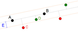
According to Definition #1 the green points are aligned to A and B because the distance between them and the dashed line linking A and B is smaller than E, and the red points are not aligned. Note the corridor defined by the two parallel lines, both at a distance from the main line equal to E.
It is very easy to define a boolean function (in R-Environment) which returns TRUE or FALSE when called with the three points and the tolerance in input:
aligned <- function(x1,y1,x2,y2,x3,y3,e)
abs((y2-y1)*x3+(x1-x2)*y3+(x2*y1-x1*y2))/sqrt((y2-y1)^2+(x1-x2)^2)<e
The aligned function gets as input: (x1,y1) first point, (x2,y2) second point, (x3,y3) point to be analysed, e tolerance.
In the previous image we want to analyse the alignment of C(89,107) and D(139,75) with A(47,79) and B(170,53) with the tolerance E=22.
By calling aligned(47,79,170,53,89,107,22) we get FALSE - as expected: the point C is not aligned to A and B.
By calling aligned(47,79,170,53,139,75,22) we get correctly TRUE: the point D is aligned to A and B.
With the function provided you have in your hands the powerful tool which draws a solid line between precise and unprecise alignments; obviously, the definition of the "correct" tolerance parameter remains the main problem(1).
Definition #2
Given a cartesian plan and two points A and B with coordinates (X1,Y1) and (X2,Y2), any C point with coordinates (XC,YC) will be "aligned" to A and B if - considering the triangle ABC - the angle in A and the angle in B are both smaller than a given tolerance E.
Also this second definition includes a tolerance parameter E, defined as an angle. Again we'll say that "C is aligned to A and B (or that A, B and C are aligned) with a tolerance equal to E degrees". In this case, the definition considers A and B as generators of three areas defined by the four lines forming an angle of E° with the line defined by A and B. Every point inside this three areas is considered "aligned" to A and B.
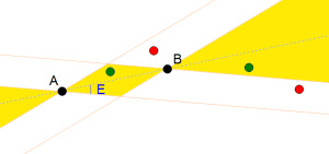
According to Definition #2 the green points are aligned to A and B because they are inside the yellow areas defined by the four lines forming an angle of E degrees with the line linking A and B. The red points are not aligned because they are out of the areas.
This second definition would solve this problem:
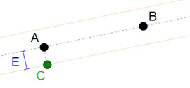
A point like C, clearly not aligned to A and B, would be considered "aligned" by definition #1. Definition #2 correctly recognise it as not aligned because - given the triangle ABC - the angle in A is 90 degrees!
It is a bit more difficult to define a boolean function which returns TRUE or FALSE when called with the three points and the tolerance in input. Firstly we should define a function calculating the angle formed by three points:
angle <- function (x1,y1,x2,y2,x3,y3)
{
   u1 <- x1-x3;
   u2 <- y1-y3;
   d1 <- x2-x3;
   d2 <- y2-y3;
   Lu <- sqrt(u1*u1 + u2*u2);
   u1 <- u1/Lu;
   u2 <- u2/Lu;
   Ld <- sqrt(d1*d1 + d2*d2);
   d1 <- d1/Ld;
   d2 <- d2/Ld;
   k <- u1*d1 + u2*d2;
   180*acos(k)/3.1415
}
angle function returns the angle in (x3,y3) (expressed in degrees from 0° to 180°) when given in input the coordinates of the other two vertices (x1,y1) and (x2,y2).
The boolean function aligned, like in definition #1, returns TRUE or FALSE if the point (x3,y3) is or not aligned to (x1,y1) and (x2,y2):
aligned <- function(x1,y1,x2,y2,x3,y3,e)
   angle(x3,y3,x1,y1,x2,y2)<e | angle(x3,y3,x2,y2,x1,y1)<e
Alignments on a line
In this analysis we'll use the first definition of alignment, so the function used will be:
aligned <- function(x1,y1,x2,y2,x3,y3,e)
abs((y2-y1)*x3+(x1-x2)*y3+(x2*y1-x1*y2))/sqrt((y2-y1)^2+(x1-x2)^2)<e
Verify an alignment within a specific area
Consider this list of coordinates (given in Comma Separated Values format, courtesy of David Williams): coordinates.csv.
Every line specifies - for each relevant item - an Id (from 1 to 100), the coordinates X and Y and a name.
You can import it in R with the function:
db<-read.csv(file="C:\\coordinates.csv",sep=";",header=T)
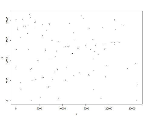
You can ask R to print the loaded map on the screen:
attach(db)
plot(x,y)
You can also add a label with the name of each point, but the result will be difficult to read!
for(i in 1:length(x)) text(x[i],y[i],name[i],cex=0.5,pos=1)
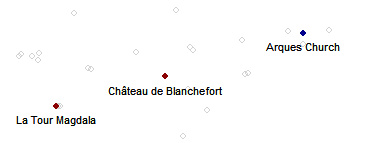
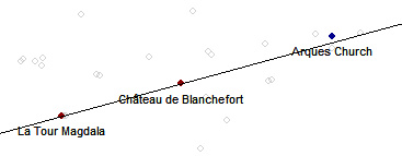
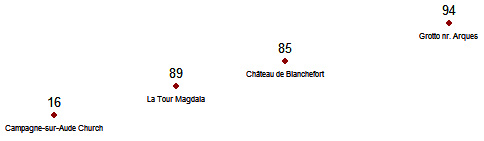
Now you can select the two key points you want to analyse, for example La Tour Magdala (Id=89) and Château de Blanchefort (Id=85).
Let's verify if it is correct that Arques Church (Id=54) is aligned to the other two points, as stated by David Wood (quoted here).
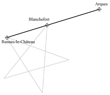
David Wood' alignment: is it correct? Let's verify it!
You define the two points and the tolerance E:
point1 <- 89
point2 <- 85
e <- 50
In order to verify the alignment we just have to ask:
aligned(x[point1],y[point1],x[point2],y[point2],x[54],y[54],e)
The answer is FALSE: they are not aligned with a tolerance 50 meters.
They are aligned if we accept an error of 210 meters: by fixing
e <- 210
the same request
aligned(x[point1],y[point1],x[point2],y[point2],x[54],y[54],e)
returns TRUE: they are aligned.
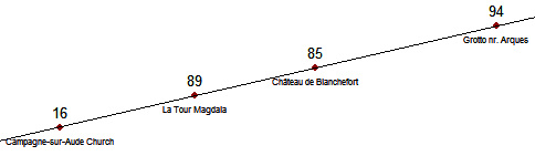
We can verify it on a map in this way:
plot(x,y,col="light gray")
points(x[point1],y[point1],pch=19,col="dark red")
points(x[point2],y[point2],pch=19,col="dark red")
points(x[54],y[54],pch=19,col="dark blue")
text(x[point1],y[point1],name[point1],cex=0.7,pos=1)
text(x[point2],y[point2],name[point2],cex=0.7,pos=1)
text(x[54],y[54],name[54],cex=0.7,pos=1)
In order to find the line passing through point 1 and point 2 we can use a linear regression. abline function draws the line through Tour Magdala and Château de Blanchefort:
z <- lm(c(y[point1],y[point2]) ~ c(x[point1],x[point2]))
abline(z)
A problem raises...
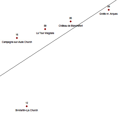
There's a problem with Definition #1: by using it, you can get paradoxical situations. They raise from the fact we are defining the corridor with the use of only two key-points - namely (x1,y1) and (x2,y2). See these points:
Let consider a tolerance of E=50. If we analyse the points 85, 89 and 94 the function aligned returns TRUE: they are aligned.
aligned(x[85],y[85],x[89],y[89],x[94],y[94],50)
TRUE
If we analyse the points 94, 89 and 16 the function aligned returns TRUE again: they are aligned.
aligned(x[94],y[94],x[89],y[89],x[16],y[16],50)
TRUE
This means that both 94 and 16 are aligned to 85 and 89. We expect a four-points alignment... but if you analyse the points 85, 89 and 16 you get FALSE!
aligned(x[85],y[85],x[89],y[89],x[16],y[16],50)
FALSE
Does the set of point (16,85,89,94) create an alignment or not? The function aligned is not able to give a definite answer. The best way would be to define a aligned function not dealing with just a couple of points but a set of n-points.
This function will be the core of the next chapter.
The "best-fit" definition
Definition #3
Given a cartesian plan and a set of points with coordinates (xn,yn) they can be considered "aligned" within a E (parameter of goodness-of-fit) if the absolute value of the correlation coefficient rxy is greater than E.
Note: rxy is the covariance of (x,y) divided by the product of the two standard deviations of x and y. R has the powerful function cor(x,y), and the two expressions give the same result:
cor(x,y)
cov(x,y)/(sqrt(var(x))*sqrt(var(y)))
In other words, given a set of n points, by calculating the correlation coefficient you can evaluate if they are someway "aligned": a value of E closer to 1 makes the alignment more precise.
The only problem raises when all the points are on an horizontal or vertical line. In this case, the correlation coefficient can not be calculated because the variance of x or y is 0; for this reason we should add the condition that if the variance of x or y is equal to 0, the points are aligned.
It is easy to define a boolean function (in R-Environment) which returns TRUE or FALSE when called with the an array of coordinates and the tolerance in input:
aligned<-function(x,y,e)
   { if(var(x)==0 | var(y)==0) TRUE else abs(cor(x,y))>e }
The function gets as input two arrays x and y containing the coordinates of the set of points and the goodness-of-fit parameter e.
Verify an alignment within a specific area (2)
Let consider again the alignment which led to a paradoxical result with Definition #1:
In order to test the function aligned we can define the two arrays of coordinates x and y (from the points 16,85,89,94):
px <- c(x[16],x[85],x[89],x[94])
py <- c(y[16],y[85],y[89],y[94])
By calling the function:
aligned(px,py,0.999)
we get TRUE: the four points are aligned within a parameter of goodness-of-fit equal to 0.999.
It doesn't raise any paradox, because the same result is obtained on subsets of the four points:
aligned(c(x[16],x[85],x[89]),c(y[16],y[85],y[89]),0.999)
aligned(c(x[16],x[85],x[94]),c(y[16],y[85],y[94]),0.999)
aligned(c(x[16],x[89],x[94]),c(y[16],y[89],y[94]),0.999)
All the three functions return correctly TRUE.
It is easy to draw the line "fitting" the set of points: just calculate the regression line (i.e. the line chosen so that it comes as close to the points as possible) and ask R to draw it:
rl <- lm(py~px)
abline(rl)
Please, download the complete R file from here bestfit.txt: you can test it on R-Environment.
Definition #4
With the method of regression line it is easy to calculate the "goodness of fit": for each point it is the perpendicular distance to the line of best fit. This could lead to a new definition of "alignment" dealing with the maximum distance tolerated E and the line of best fit:
Given a cartesian plan and a set of points with coordinates (xn,yn) they can be considered "aligned" with a tolerance E if - calculated the regression line which best fits the points, each point has a distance from that line smaller than E.
In other words, given a set of n points you can always calculate the inclination (m) and the intercept (q) of the regression line best fitting the set: the points are "aligned" if the perpendicular distance between each (x,y) from the line y=mx+q is smaller than E.
The function is easily defined. Firstly we define a function calculating the distance between a point and a line:
distance<-function(x,y,m,q) { abs((y-m*x-q)/sqrt(m^2+1)) }Then we create the boolean aligned in this way:
aligned <- function(x,y,e)
{
  rl <- lm(y~x);
  m <- as.numeric(rl[[1]][2]);
  q <- as.numeric(rl[[1]][1]);
  d <- distance(x,y,m,q)<e;
  tmp <- TRUE;
  for(i in d) tmp <- tmp & i;
  tmp
}
This function is more "user friendly": the input is the same as the aligned function according to Definition #3, but it is easier to fix the value of E, being in the same measurement unit of the coordinates. So if your coordinates are in meters, also E is in meters.
By using the latter definition of aligned, you can call:
aligned(px,py,25)
TRUE
It returns TRUE, so we can say that these four points:
are at a distance from the line smaller than 25 meters. In order to get the exact distances from the best fit line you can define a new function:
distances <- function(x,y)
{
  rl <- lm(y~x);
  m <- as.numeric(rl[[1]][2]);
  q <- as.numeric(rl[[1]][1]);
  distance(x,y,m,q)
}
By calling it with the x and y arrays of coordinates, it returns an array of distances from the regression line:
distances(px,py)
13.758366  5.419433 23.150012  3.972212
The point 16 is 13.76 units from the line, the point 85 is 5.42 units from the line and so on.
It gives no information about the alignment; you have to test if the distances are all smaller than E: if so, they are aligned with a tolerance E.
This leads to an interesting point: there is a best fit line for each set of points. By adding the point 12 to the list:
px <- c(px,x[12])
py <- c(py,y[12])
we can draw the new regression line:
rl <- lm(py~px)
abline(rl)
and the distances are clearly greater than before:
distances(px,py)
3365.7148 1036.0479 2164.4213  629.8708 5936.3132
The result should be read keeping in mind the order of points defined: 16, 85, 89, 94 and 12. So the point 12 is at a distance of 5936.31 units from the regression line.
By defining a E=6000, they can be positively considered aligned (!):
aligned(px,py,6000)
TRUE
Please, download the complete R file from here bestfit2.txt: you can test it on R-Environment.
How to find all alignments
With functions #3 and #4 it is not difficult to scan a set of points in order to find all the alignments. The problem is to optimize the scanning procedure, because the "brute force" approach is not the best one. The complexity of any "brute force" algorithm would be exponential; some facts will help in the definition of the best algorithm:
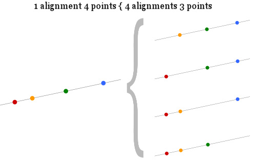
1) A set of N points generates at least N*(N-1)/2 "trivial" alignments of two points.
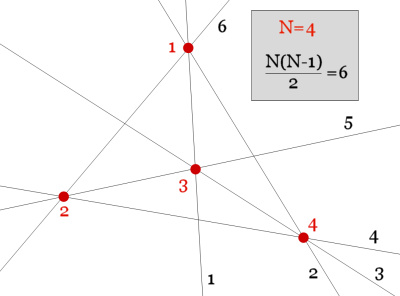
2) If M points are aligned, the same set represents a number of M alignments of M-1 points. (For example: 4 points aligned A,B,C,D represent also 4 alignment of three points each: A,B,C and A,B,D and A,C,D and B,C,D)
By these two points we can define an algorithm with quadratic complexity:
1) Define a set of alignments of 2 points by using all the possible N*(N-1)/2 pairs of points;
2) In order to look for all the alignments of 3 points, for each of the N*(N-1)/2 alignments of 2 points verify if any of the other points are aligned with the 2. All the points aligned to each pair generate a 3 points alignment.
3) In order to look for all the alignments of 4 points, for each of the M alignments of 3 points (found at step 2) verify if any of the other points are aligned with the 3. All the points aligned to each pair generate a 4 points alignment.
...
N) The algorithm stops when no N+1 points alignment is found.
A useful trick can be added: in order to define the alignments to be tested, I have to create an array of points. Thanks to the property of "commutativity" of the points verified with the function aligned - and in order to avoid a double verification of the same set of points shuffled (for example 1,2,3 and 3,1,2) - whenever I define a set of points, I limit myself to the sorted one (so I will verify only the set 1,2,3).
Note that this can be performed only because we use Definition #3 or Definition #4: "commutativity" is not a property of Definition #1 and #2!
Please, download the complete R file from here find_all.txt: you can test it on R-Environment.
Alignments on a circle
In order to evaluate the points aligned on a circle defined by a center (point 1) and a radius (the distance between point 1 and point 2) we need a new function returning the distance between two points (x1,y1) and (x2,y2):
distance <- function(x1,y1,x2,y2) sqrt((x1-x2)^2+(y1-y2)^2)
A second function will return TRUE or FALSE when called with a third point as a parameter when it is near the circle with a tolerance equal to E:
aligned <- function(x1,y1,x2,y2,x3,y3,e)
abs(distance(x1,y1,x2,y2)-distance(x1,y1,x3,y3))<e
In this function (x1,y1) is the center of the circle, the distance between (x1,y1) and (x2,y2) is the radius and (x3,y3) is the point to be tested.
It is easy to scan all the remaining points in order to find the ones "aligned" on the circle.
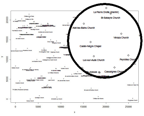
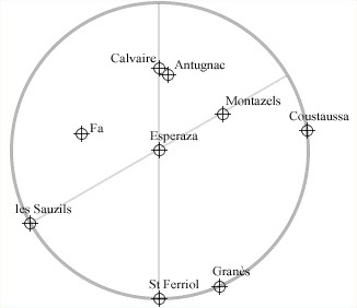
Let's verify if it is correct that Esperaza is the center of a circle passing through Coustaussa, Granès, Saint Ferriol and Les Sauzils, as stated by Henry Lincoln (quoted here).
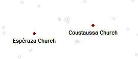
Now you can select two key points you want to analyse, for example Esperaza (Id=35) and Coustaussa (Id=47).
You define the two points and the tolerance E (10 meters):
point1 <- 35
point2 <- 47
e <- 10
Then you start to draw the map and the two defining point:
plot(x,y,col="light gray")
points(x[point1],y[point1],pch=19,col="dark red")
points(x[point2],y[point2],pch=19,col="dark red")
text(x[point1],y[point1],name[point1],cex=0.7,pos=1)
text(x[point2],y[point2],name[point2],cex=0.7,pos=1)
By scanning all the 98 points, you can find the ones lying on the circle:
for(i in 1:length(x))
{
  if(i!=point1 & i!=point2)
  if(aligned(x[point1],y[point1],x[point2],y[point2],x[i],y[i],e))
  {
    points(x[i],y[i],pch=19,col="dark blue")
    text(x[i],y[i],name[i],cex=0.5,pos=1)
  }
}
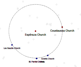
As stated by Henry Lincoln, the alignment of Granès, Saint Ferriol and Les Sauzils on the circle is correct within a tolerance of 50 meters.
Please, download the complete R file from here: circle.txt
Alignments on pentacles
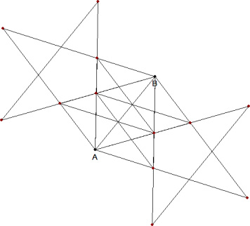
Two points define four different pentacles. Given the coordinates of the first two points (A1,A2) and (B1,B2), with a simple mathematical formula it is possible to find the coordinates of the three other vertices in the pentacles.
Let's fix the first two points A(10,10) and B(40,50):
A1 <- 10
A2 <- 10
B1 <- 40
B2 <- 50
The other points can be calculated with these formulas:
C1<-(B1-A1)*((sqrt(5)-1)/4)+(B2-A2)*sqrt(sqrt(5)/8+5/8)+B1
C2<-(-1)*(B1-A1)*sqrt(sqrt(5)/8+(5/8))+(B2-A2)*((sqrt(5)-1)/4)+B2
D1<-(C1-B1)*((sqrt(5)-1)/4)+(C2-B2)*sqrt(sqrt(5)/8+5/8)+C1
D2<-(-1)*(C1-B1)*sqrt(sqrt(5)/8+(5/8))+(C2-B2)*((sqrt(5)-1)/4)+C2
E1<-(D1-C1)*((sqrt(5)-1)/4)+(D2-C2)*sqrt(sqrt(5)/8+5/8)+D1
E2<-(-1)*(D1-C1)*sqrt(sqrt(5)/8+(5/8))+(D2-C2)*((sqrt(5)-1)/4)+D2
The five points should be stored in an array:
x1 <- c(A1,C1,E1,B1,D1)
y1 <- c(A2,C2,E2,B2,D2)
A second pentacle can be found with a second formula:
C1<-(A1-B1)*((sqrt(5)-1)/4)+(A2-B2)*sqrt(sqrt(5)/8+5/8)+A1
C2<-(-1)*(A1-B1)*sqrt(sqrt(5)/8+(5/8))+(A2-B2)*((sqrt(5)-1)/4)+A2
D1<-(C1-A1)*((sqrt(5)-1)/4)+(C2-A2)*sqrt(sqrt(5)/8+5/8)+C1
D2<-(-1)*(C1-A1)*sqrt(sqrt(5)/8+(5/8))+(C2-A2)*((sqrt(5)-1)/4)+C2
E1<-(D1-C1)*((sqrt(5)-1)/4)+(D2-C2)*sqrt(sqrt(5)/8+5/8)+D1
E2<-(-1)*(D1-C1)*sqrt(sqrt(5)/8+(5/8))+(D2-C2)*((sqrt(5)-1)/4)+D2
The five points should be again stored in a second array:
x2 <- c(B1,C1,E1,A1,D1)
y2 <- c(B2,C2,E2,A2,D2)
The third and fourth pentacles can be calcualted with these two formulas:
C1<-B1-(1+sqrt(5))*(B1-A1)/4-sqrt((5-sqrt(5))/2)*(B2-A2)/2
C2<-sqrt((5-sqrt(5))/2)*(B1-A1)/2+B2-(1+sqrt(5))*(B2-A2)/4
D1<-C1-(1+sqrt(5))*(C1-B1)/4-sqrt((5-sqrt(5))/2)*(C2-B2)/2
D2<-sqrt((5-sqrt(5))/2)*(C1-B1)/2+C2-(1+sqrt(5))*(C2-B2)/4
E1<-D1-(1+sqrt(5))*(D1-C1)/4-sqrt((5-sqrt(5))/2)*(D2-C2)/2
E2<-sqrt((5-sqrt(5))/2)*(D1-C1)/2+D2-(1+sqrt(5))*(D2-C2)/4
x3 <- c(A1,B1,C1,D1,E1)
y3 <- c(A2,B2,C2,D2,E2)

C1<-A1-(1+sqrt(5))*(A1-B1)/4-sqrt((5-sqrt(5))/2)*(A2-B2)/2
C2<-sqrt((5-sqrt(5))/2)*(A1-B1)/2+A2-(1+sqrt(5))*(A2-B2)/4
D1<-C1-(1+sqrt(5))*(C1-A1)/4-sqrt((5-sqrt(5))/2)*(C2-A2)/2
D2<-sqrt((5-sqrt(5))/2)*(C1-A1)/2+C2-(1+sqrt(5))*(C2-A2)/4
E1<-D1-(1+sqrt(5))*(D1-C1)/4-sqrt((5-sqrt(5))/2)*(D2-C2)/2
E2<-sqrt((5-sqrt(5))/2)*(D1-C1)/2+D2-(1+sqrt(5))*(D2-C2)/4
x4 <- c(B1,A1,C1,D1,E1)
y4 <- c(B2,A2,C2,D2,E2)
In order to print the result, let's fix the two source points:
plot(c(x1,x2,x3,x4),c(y1,y2,y3,y4),col="light gray")
points(A1,A2,pch=19)
points(B1,B2,pch=19)
text(A1,A2,"A",pos=1)
text(B1,B2,"B",pos=1)
The four pentacles can be easily drawn with the function polygon:
polygon(x1,y1)
polygon(x2,y2)
polygon(x3,y3)
polygon(x4,y4)
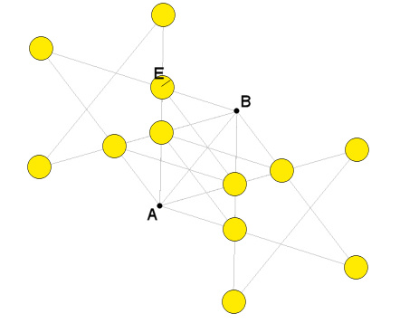
Excluding the two source points, we have a total of 12 points on the vertices of the pentacles. The list of them can be stored in an array and printed:
vx<-c(x1[2],x1[3],x1[5],x2[2],x2[3],x2[5],x3[3],x3[4],x3[5],x4[3],x4[4],x4[5])
vy<-c(y1[2],y1[3],y1[5],y2[2],y2[3],y2[5],y3[3],y3[4],y3[5],y4[3],y4[4],y4[5])
points(vx,vy,col="dark red",pch=19)
Any point at a distance from one of these 12 points smaller than a tolerance value E can be considered "on a pentacle" defined by the two points A and B.
Please, download the complete R file from here: pentacle.txt
Using these formulas, a function aligned can be defined to verify if the point (C1,C2) is on a vertex of a pentacle defined by points (A1,A2) and (B1,B2). The function can be downloaded from here: pentacle_aligned.txt
This function recognises as "aligned" to A&B-generated-pentacles all the points inside the yellow circular areas, each of which has a radius equal to E:
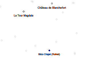
By using this function on Rennes-le-Château map and selecting La Tour Magdala and the Château de Blanchefort, with a tolerance of 400 meters (!) you can identify a unique point fitting one pentacle, the Bezu Chapel:
_________________
(1) Is there any "correct" value for E? Obviously not: every point could be considered "aligned" to A and B, when you fix a E value greater than the distance between the point and the line defined by A and B!