
«Existence is exalting, as once curiosity is awakened; this exercise of curiosity transforms life into a poetic adventure.»
(Louis Pauwels & Jacques Bergier)
“Timewave zero” is a numerological formula created by Terence McKenna which allegedly correlates time and history with the ebb and flow of something called “Novelty”, claimed to be a quality intrinsic to the temporal structure of the universe, a measurement of universe’s interconnectedness (or “organised complexity”) over time: when its value increases, the amount of “novelty” decreases; the function will reach “zero” on 2012, the teleological attractor point of history, the singularity of infinite complexity.
According to McKenna,
all phenomena are at root constellated by a wave form which is the hierarchical summation of its constituent parts, morphogenetic patterns related to those in DNA. [...] We argue that the theory of the hyperspatial nature of superconductive bonds, and the experiment we devised to test that theory, yielded [...] a modular wave-hierarchy theory of the nature of time that we have been able to construe, using a particular mathematical treatment of the I Ching, into a general theory of systems, which illuminates the nature of time and organism and provides an idea model which explains the interconnection of physical and psychological phenomena from the submolecular to the macrocosmic level. (1)
Terence McKenna affirmed also that the graph appears to show big variations of novelty corresponding with great shifts in humanity’s cultural and biological evolution.
The theory of Timewave Zero was revealed to McKenna in the wake of an unusual psychedelic experiment conducted deep in the Amazon jungle in Colombia in 1971, which led to his being instructed in certain transformations of numbers, derived from the “King Wen Sequence” of I Ching hexagrams, relating to the occurrence of temporal phenomena. The “King Wen Sequence” has been translated into an array of 384 integer values (the process is available here) used as the “seed” of the Timewave Zero function.
From a mathematical point of view, it is a fractal function where each point is calculated as the sum of a doubly infinite series.
Let v(x) be a function equal to 0 for all x less than B and whose value is always finite (less than a given C).
Having defined such a function, we can define its “fractal transform” this way:
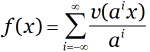
Timewave Zero function is the “fractal transform” of a saw-tooth function.
Consider this list of 384 values derived from a transformation of “King Wen Sequence”:
0, 0, 0, 2, 7, 4, 3, 2, 6, 8, 13, 5, 26, 25, 24, 15, 13, 16, 14, 19, 17, 24, 20, 25, 63, 60, 56, 55, 47, 53, 36, 38, 39, 43, 39, 35, 22, 24, 22, 21, 29, 30, 27, 26, 26, 21, 23, 19, 57, 62, 61, 55, 57, 57, 35, 50, 40, 29, 28, 26, 50, 51, 52, 61, 60, 60, 42, 42, 43, 43, 42, 41, 45, 41, 46, 23, 35, 34, 21, 21, 19, 51, 40, 49, 29, 29, 31, 40, 36, 33, 29, 26, 30, 16, 18, 14, 66, 64, 64, 56, 53, 57, 49, 51, 47, 44, 46, 47, 56, 51, 53, 25, 37, 30, 31, 28, 30, 36, 35, 22, 28, 32, 27, 32, 34, 35, 52, 49, 48, 51, 51, 53, 40, 43, 42, 26, 30, 28, 55, 41, 53, 52, 51, 47, 61, 64, 65, 39, 41, 41, 22, 21, 23, 43, 41, 38, 24, 22, 24, 14, 17, 19, 52, 50, 47, 42, 40, 42, 26, 27, 27, 34, 38, 33, 44, 44, 42, 41, 40, 37, 33, 31, 26, 44, 34, 38, 46, 44, 44, 36, 37, 34, 36, 36, 36, 38, 43, 38, 27, 26, 30, 32, 37, 29, 50, 49, 48, 29, 37, 36, 10, 19, 17, 24, 20, 25, 53, 52, 50, 53, 57, 55, 34, 44, 45, 13, 9, 5, 34, 26, 32, 31, 41, 42, 31, 32, 30, 21, 19, 23, 43, 36, 31, 47, 45, 43, 47, 62, 52, 41, 36, 38, 46, 47, 40, 43, 42, 42, 36, 38, 43, 53, 52, 53, 47, 49, 48, 47, 41, 44, 15, 11, 19, 51, 40, 49, 23, 23, 25, 34, 30, 27, 7, 4, 4, 32, 22, 32, 68, 70, 66, 68, 79, 71, 43, 45, 41, 38, 40, 41, 24, 25, 23, 35, 33, 38, 43, 50, 48, 18, 17, 26, 34, 38, 33, 38, 40, 41, 34, 31, 30, 33, 33, 35, 28, 23, 22, 26, 30, 26, 75, 77, 71, 62, 63, 63, 37, 40, 41, 49, 47, 51, 32, 37, 33, 49, 47, 44, 32, 38, 28, 38, 39, 37, 22, 20, 17, 44, 50, 40, 32, 33, 33, 40, 44, 39, 32, 32, 40, 39, 34, 41, 33, 33, 32, 32, 38, 36, 22, 20, 20, 12, 13, 10
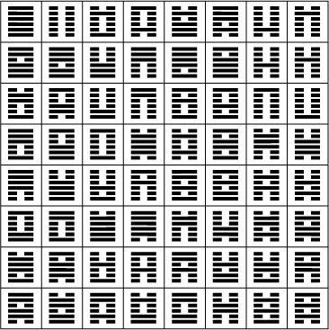
King Wen Sequence
These numbers provide the basic numerical values used in the definition of a w(i) function, defined as the i-th value of this set, using zero-based indexing:
w(0)=0, w(1)=0, w(2)=0, w(3)=2, w(4)=7 and so on.
In order to extend w(i) to values of i greater than 383, we can simply define a new function W(i)=w(i mod 384) where i mod 384 is the remainder upon division of i by 384.
Thus for example W(777)=w(777 mod 384)=v(9)=8.
Note that W() is a discrete function defined only for integers, not for all real numbers: in order to extend it for any non-negative real numbers x we can easily define a new v(x) function as the linear interpolation between the values W(int(x)) and W(int(x)+1), where int(x) is the integral part of x. Formally, v(x) is defined as:
v(x) = W(int(x)) + (x – int(x)) × (W(x+1) – W(x))
Timewave Zero function is the fractal transform of v(x) using a=64, divided per 64^3:
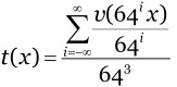
where x = time in days prior to 6 AM on the zero date. Thus the value of Timewave Zero on the zero date is:
t(0) = f(0) / 64^3 = 0
The day before the zero date is:
t(1) = f(1) / 64^3 = 0.0000036160151
and so on.
These values are independent of the actual zero date, for which McKenna arbitrarily chose december 21th, 2012.
The analysis of Timewave Zero function is easy with R programming language. This is the definition of W(x) function:
W <-function(x)
{
	datapoint <- c(0, 0, 0, 2, 7, 4, 3, 2, 6, 8, 13, 5, 26, 25, 24, 15,
	13, 16, 14, 19, 17, 24, 20, 25, 63, 60, 56, 55, 47, 53, 36, 38, 39,
	43, 39, 35, 22, 24, 22, 21, 29, 30, 27, 26, 26, 21, 23, 19, 57, 62,
	61, 55, 57, 57, 35, 50, 40, 29, 28, 26, 50, 51, 52, 61, 60, 60, 42,
	42, 43, 43, 42, 41, 45, 41, 46, 23, 35, 34, 21, 21, 19, 51, 40, 49,
	29, 29, 31, 40, 36, 33, 29, 26, 30, 16, 18, 14, 66, 64, 64, 56, 53,
	57, 49, 51, 47, 44, 46, 47, 56, 51, 53, 25, 37, 30, 31, 28, 30, 36,
	35, 22, 28, 32, 27, 32, 34, 35, 52, 49, 48, 51, 51, 53, 40, 43, 42,
	26, 30, 28, 55, 41, 53, 52, 51, 47, 61, 64, 65, 39, 41, 41, 22, 21,
	23, 43, 41, 38, 24, 22, 24, 14, 17, 19, 52, 50, 47, 42, 40, 42, 26,
	27, 27, 34, 38, 33, 44, 44, 42, 41, 40, 37, 33, 31, 26, 44, 34, 38,
	 6, 44, 44, 36, 37, 34, 36, 36, 36, 38, 43, 38, 27, 26, 30, 32, 37,
	29, 50, 49, 48, 29, 37, 36, 10, 19, 17, 24, 20, 25, 53, 52, 50, 53,
	57, 55, 34, 44, 45, 13,  9,  5, 34, 26, 32, 31, 41, 42, 31, 32, 30,
	21, 19, 23, 43, 36, 31, 47, 45, 43, 47, 62, 52, 41, 36, 38, 46, 47,
	40, 43, 42, 42, 36, 38, 43, 53, 52, 53, 47, 49, 48, 47, 41, 44, 15,
	11, 19, 51, 40, 49, 23, 23, 25, 34, 30, 27,  7,  4,  4, 32, 22, 32,
	68, 70, 66, 68, 79, 71, 43, 45, 41, 38, 40, 41, 24, 25, 23, 35, 33,
	38, 43, 50, 48, 18, 17, 26, 34, 38, 33, 38, 40, 41, 34, 31, 30, 33,
	33, 35, 28, 23, 22, 26, 30, 26, 75, 77, 71, 62, 63, 63, 37, 40, 41,
	49, 47, 51, 32, 37, 33, 49, 47, 44, 32, 38, 28, 38, 39, 37, 22, 20,
	17, 44, 50, 40, 32, 33, 33, 40, 44, 39, 32, 32, 40, 39, 34, 41, 33,
	33, 32, 32, 38, 36, 22, 20, 20, 12, 13, 10);
	datapoint[x%%length(datapoint)+1]
}
This is the definition of the interpolated v(x) function:
v <- function(x)
{
	W(floor(x))+(x-floor(x))*(W(x+1)-W(x));
}
Timewave Zero function is simply:
t <- function(x)
{
   temp<-0;
   for(i in c(-5:5)) temp<-temp+((64^i)*v(x/(64^i)));
   temp/(64^3)
}
In order to feed t(x) you need to convert a date expressed in the form m/d/y into an integer with this function:
day <- function(m,d,y)
{
  base<-as.integer(floor(unclass(ISOdatetime(2012,12,21,6,0,0))/86400));
  result<-base-as.integer(floor(unclass(ISOdatetime(y,m,d,6,0,0))/86400));
  if(result>0) { result } else { 0 };
}
Timewave Zero value for September 11th, 2001 can be calculated this way:
t(day(9,11,2001))
The result is
0.01500575
which is the amount of novelty on that day. According to McKenna definition, on December 21th, 2012 the amount of novelty:
t(day(12,21,2012))
will be equal to:
0
With this function you can plot the chart for any month:
month<-function(m,y)
{
  MONTH<-c("January","February","March","April","May","June","July",
   “August”,“September”,“October”,“November”,“December”);
  timewave<-c();
  for(d in c(1:30))
    timewave<-c(timewave,t(day(m,d,y)));
  plot(timewave,type=“l”,lab=c(30,10,10), main = “Timewave Zero function”,
    xaxt=“n”,xlab=paste(MONTH[m],y),ylab=“”);
  axis(1, 1:30);
}
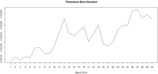
The chart of the month of March 2010 can be plotted this way:
month(3,2010)
and the result will be:
With this function you can plot the chart for any year:
year<-function(y)
{
  start<-day(1,1,y)
  end<-day(12,31,y)
  timewave<-c();
  for(d in c(start:end))
    timewave<-c(timewave,t(d));
  plot(timewave,type=“l”,lab=c(12,10,10),
    main = “Timewave Zero function”,xaxt=“n”,xlab=y,ylab=“”);
  axis(1, c(0,31,59,90,120,151,181,212,243,273,304,334,365),
    c(“Jan”,“Feb”,“Mar”,“Apr”,“May”,“Jun”,
    “Jul”,“Aug”,“Sep”,“Oct”,“Nov”,“Dec”,“Jan”));
}
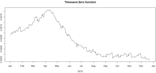
The chart of the year 2012 can be plotted this way:
year(2012)
and the result will be:
1. Dennis and Terence McKenna, The Invisible Landscape, 1975, pages 101-103.
BY-NC-SA 4.0 • Attribution-NonCommercial-ShareAlike 4.0 International